Statistics homework 9
Theory:
-
What is the “Brownian motion” and what is a Wiener process. History, importance, definition and applications (Bachelier, Wiener, Einstein, …):
-
An “analog” of the CLT for stochastic process: the standard Wiener process as “scaling limit” of a random walk and the functional CLT (Donsker theorem) or invariance principle. Explain the intuitive meaning of this result and how you have already illustrated the result in your homework.
Practice:
-
Discover one of the most important stochastic process by yourself ! Consider the general scheme we have used so far to simulate stochastic processes (such as the relative frequency of success in a sequence of trials, the sample mean, the random walk, the Poisson point process, etc.) and now add this new process to our simulator. Starting from value 0 at time 0, for each of m paths, at each new time compute P(t) = P(t-1) + Random step(t), for t = 1, …, n, where the Random step(t) is now: σ * sqrt(1/n) * Z(t), where Z(t) is a N(0,1) random variable (the “diffusion” σ is a user parameter, to scale the process dispersion). At time n (last time) and one (or more) other chosen inner time 1<j<n (j is a program parameter) create and represent with histogram the distribution of P(t). Observe the behavior of the process for large n.
-
Create the a distribution representation (histogram, or CDF …) to represent the following:
- Realizations taken from a Normal(0,1)
- Realizations of the mean, obtained by averaging several times (say m times, m large) n of the above realizations
- Realizations of the variance, obtained by averaging several times (say m times, m large) n of the above realizations
- Realizations taken from exp(N(0,1)))
- Realizations taken from N(0,1) squared
- Realizations taken from a (squared N(0,1)) divided by another (squared N(0,1))
Practice theory: Try to find on the web what are the names of the random variables that you just simulated in the applications, and see if the means and variances that you obtain in the simulation are compatible with the “theory”. If not fix the possible bugs.
Theory 1
Brownian motion
The Brownian motion is the random motion of particles suspended in a fluid medium.
As said in [1] this pattern of motion typically consists of random fluctuations in a particle’s position inside a fluid subdomain, followed by a relocation to another subdomain. Each relocation is followed by more fluctuations within the new closed volume. This pattern describes a fluid at thermal equilibrium, defined by a given temperature.
Studied for the first time by the botanist Robert Brown in 1827 observing on the microscope the motion of pollen immersed in water. Eight years later, Albert Einstein published a paper where he modeled the motion of the pollen particles as being moved by individual water molecules.
The direction of the force of atomic bombardment is constantly changing, and at different times the particle is hit more on one side than another, leading to the seemingly random nature of the motion.
Einstein’s theory
There are two parts to Einstein’s theory: the first part consist in formulation of a diffusion equation for Brownian particles, and the second part consist in relating the diffusion coefficient to measurable physical quantities.
The first part of Einstein’s argument was to determine how far a Brownian particle travels in a given time interval. Assuming that N particles start from the origin at the initial time t = 0, the diffusion equation has the solution:
\[\rho(x, t) = \frac{N}{\sqrt{4\pi Dt}}e^{-\frac{x^{2}}{4Dt}}\]Which is a normal distribution with mean 0 and variance $2Dt$. From this equation, Einstein extracted the moments and argued that the displacement of a Brownian particle is not proportional to the elapsed time, but rather to its square root.
Wiener process
As described in [2] the Wiener process is a real valued continuous-time stochastic process named in honor of American mathematician Norbert Wiener for his investigations on the mathematical properties of the one-dimensional Brownian motion. It is often also called Brownian motion due to its historical connection with the physical process.
The Wiener process \(W_{t}\) is characterized by the following properties:
- \[W_{0}=0\]
- \(W\) has independent increments: for every \(t>0\), the future increments \(W_{t+u}-W_{t}\), \(u \ge 0\), are independent of the past values \(W_{s}\), \(s \le t\)
- \(W\) has Gaussian increments: \(W_{t+u}-W_{t}\) is normally distributed with mean \(0\) and variance \(u\), \(W_{t+u}-W_{t}\sim {\mathcal{N}}(0,u)\).
- \(W\) has continuous paths: \(W_{t}\) is continuous in \(t\).
Applications
- In physics, it is used to study Brownian motion
- In applied mathematics, the Wiener process is used to represent the integral of a white noise Gaussian process, useful to model the noise in electronics engineering
- It also forms the basis for the rigorous path integral formulation of quantum mechanics
- It is also prominent in the mathematical theory of finance, in particular the Black–Scholes option pricing model
[1] https://en.wikipedia.org/wiki/Brownian_motion
[2] https://en.wikipedia.org/wiki/Wiener_process
Theory 2
The intuitive meaning of the Donsker theorem and the the standard Wiener process as “scaling limit” of a random walk is that every random walk with a step that varies according to a certain distribution tends to a standard brownian motion as the step size decreases. In the second application of homework 7 we shoewd it.
Practice 1
How it works
Practice 2
How it works
Download projects
Practice theory
Let \(Z \sim {\mathcal{N}}(0,u)\)
-
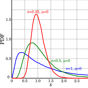
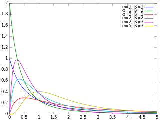
\(e^{Z}\) is a log-normal distribution [1]

-
\(Z^{2}\) is a chi squared distribution [2]

-
\(\frac{Z^{2}}{Z^{2}}\) is a beta prime distribution [3]

[1] https://en.wikipedia.org/wiki/Log-normal_distribution